3. Example of usage

This example will show how to monitor a DDS network using DDS Monitor and how to understand the different application features and configurations.

3.1. Fast DDS with Statistics module

In order to show the DDS Monitor application running and monitoring a real DDS network, this tutorial uses a Fast DDS example to create a simple and understandable DDS network. The example proposed by this tutorial uses the hello_world example of Fast DDS repository.

In order to execute this minimum DDS scenario where each entity publishes its statistical data, follow these steps:

1. Compile Fast DDS library with CMake option COMPILE_EXAMPLES to build the examples (-DCOMPILE_EXAMPLES=ON).

2. Have DDS Monitor installed or a working environment with Fast DDS, Fast DDS Statistics Backend and DDS Monitor built.

3. Use the environment variable FASTDDS_STATISTICS to activate the statistics writers in the DDS execution (see following section).

For further information about the Statistics configuration, please refer to Fast DDS statistics module. For further information about installation of the Monitor and its dependencies, please refer to the documentation section DDS Monitor on Linux or Linux installation from sources.

3.1.1. Hello World Example

For this tutorial, the Fast DDS hello_world example is used to create a simple DDS network to be monitored. Below are the commands executed in order to run this network. Note that this tutorial does not start with this DDS network running, and it is instead executed once the monitor has been started. This does not change the Monitor behavior, but would change the data and information shown by the application.

1. Execute a Fast DDS hello_world subscriber with statistics data active.

   export FASTDDS_STATISTICS="HISTORY_LATENCY_TOPIC;NETWORK_LATENCY_TOPIC;\
   PUBLICATION_THROUGHPUT_TOPIC;SUBSCRIPTION_THROUGHPUT_TOPIC;RTPS_SENT_TOPIC;\
   RTPS_LOST_TOPIC;HEARTBEAT_COUNT_TOPIC;ACKNACK_COUNT_TOPIC;NACKFRAG_COUNT_TOPIC;\
   GAP_COUNT_TOPIC;DATA_COUNT_TOPIC;RESENT_DATAS_TOPIC;SAMPLE_DATAS_TOPIC;\
   PDP_PACKETS_TOPIC;EDP_PACKETS_TOPIC;DISCOVERY_TOPIC;PHYSICAL_DATA_TOPIC;\
   MONITOR_SERVICE_TOPIC"
   
   ./build/fastdds/examples/cpp/hello_world/hello_world subscriber
   

   where subscriber argument creates a DomainParticipant with a DataReader in the topic hello_world_topic in Domain 0.

2. Execute a Fast DDS hello_world publisher with statistics data active.

   export FASTDDS_STATISTICS="HISTORY_LATENCY_TOPIC;NETWORK_LATENCY_TOPIC;\
   PUBLICATION_THROUGHPUT_TOPIC;SUBSCRIPTION_THROUGHPUT_TOPIC;RTPS_SENT_TOPIC;\
   RTPS_LOST_TOPIC;HEARTBEAT_COUNT_TOPIC;ACKNACK_COUNT_TOPIC;NACKFRAG_COUNT_TOPIC;\
   GAP_COUNT_TOPIC;DATA_COUNT_TOPIC;RESENT_DATAS_TOPIC;SAMPLE_DATAS_TOPIC;\
   PDP_PACKETS_TOPIC;EDP_PACKETS_TOPIC;DISCOVERY_TOPIC;PHYSICAL_DATA_TOPIC;\
   MONITOR_SERVICE_TOPIC"
   
   ./build/fastdds/examples/cpp/hello_world/hello_world publisher --samples 0
   

   where publisher argument creates a DomainParticipant with a DataWriter in the topic hello_world_topic in Domain 0. The following arguments indicate this process to run until the user press enter (0 samples) and to write a message every tenth of a second (100 milliseconds period).

The environment variable FASTDDS_STATISTICS activates the statistics writers for a Fast DDS application execution. This means that the DomainParticipants created within this variable will report the statistical data related to them and their sub-entities.

Please refer to Fast DDS documentation for further information about the available statistical topics.

3.2. DDS Monitor Execution

The following section presents a complete DDS Monitor execution, monitoring a real DDS network.

3.2.1. Initial Window

The Monitor starts with no DDS entities running. First of all, the DDS Monitor initial window is shown. Press Start monitoring! in order to enter the application and start the monitoring.

3.2.2. Initiate monitoring

Once in the application, the first dialog that appears asks the user to enter a domain to begin monitoring it. Monitoring a domain means to listen in that domain for DDS entities that are running and reporting statistical data. Please refer to section Monitor Domain for further information.

First, the Cancel button is pressed so the user can see around the monitor and check its configurations, but no entities or data will be shown as there are no domains being monitored. You can always return to the Initialize Monitoring dialog from File.

Let’s initialize monitoring in domain 0 and pressing OK.

3.2.3. Add physical and logical panels

By default, the Monitor only displays the DDS panel which lists the DDS entities together with their configuration and available statistics information. In order to open the logical and the physical panels, click on the top right corner of the Explorer Panel, in button ··· and add all the panels to visualize the whole information.

At this point, you are going to see the whole window of the application. You should be able to see how an unique entity is present in the application in the left sidebar. This is the domain that you have just initiated. Once a domain is initiated, it is set as Selected Entity and so its information is shown in the Entity Info Panel.

For specific details on how the information is divided and where to find it, please refer to DDS Monitor Basic.

3.2.4. Execute subscriber

Now, execute the first DDS entity in our DDS network: a DomainParticipant with one DataReader in topic hello_world_topic in domain 0 following the steps given in Hello World Example. Once the subscriber is running our window will update and you could see new information in the left sidebar.

First of all, the number of entities discovered has increased. Now, you have a DomainParticipant called RTPSParticipant, holding a DataReader called hello_world_topic_0.0.1.4. This DataReader has a locator, which will be the Shared Memory Transport locator. That is because the Monitor and the DomainParticipant are running in the same host, and so they communicate using the Shared Memory Transport (SHM) protocol.

You should be able to see as well that now Host exists, with a User and a Process where RTPSParticipant is running. This information is retrieved by the DomainParticipant thanks to activating the PHYSICAL_DATA_TOPIC. There is also a new Topic hello_world_topic under Domain 0.

Double-clicking any entity name shows its specific information, such as name, backend id, QoS, etc.

3.2.5. Execute publisher

The next step is to execute a publisher in topic hello_world_topic in domain 0, following the steps given in Hello World Example. Once the publisher is running you will see that new entities have appeared. Specifically, a new DomainParticipant also called RTPSParticipant with a DataWriter hello_world_topic_0.0.1.3 and, in the case that this publisher has been executed from same Host and User, there will be a new Process that represents the process where this new RTPSParticipant is running.

3.2.6. Domain View

Now that we have both our publisher and subscriber in execution, we can check the configuration of the DDS network that has just been created. Click on Domain View in the Main Panel to open the Domain display. In this tab, we can see a graph describing the structure of our network: our single Host contains our single User, which in turn contains both our Processes. Each Process is related to one of our Participants, either the publisher or the subscriber. It’s easy to distinguish them in this view: with the vertical line representing our Topic, the publisher contains the DataWriter, represented with an arrow that feeds into the Topic, while the subscriber contains the DataReader, represented with an arrow coming from the Topic.

In this view, we have access to different functionalities, including filtering by Topic (right-click over the Topic name, and choose Filter topic graph, opening the filtered graph in a new Tab). Additionally, we can access the IDL representation of any of the Topics, by pressing right-click over the Topic name, and choosing Data type IDL view. This opens a new Tab with the required information, which can be copied and pasted.

Since we’re not going to be using these Tabs anymore, click on the X to close all Tabs and return to the New Tab view.

3.2.7. Summary of Statistical Data

In Statistics Panel you can see the main information retrieved by each entity. This panel shows a summary of the data retrieved by the entity that is clicked. In this case, you could only see the data that the entities are publishing, and the rest of DataKinds that are related to the topics that we are not using will remain without data.

3.2.8. Change entity alias

In order to make the user experience easier, it is allowed to change the name of any specific entity. Change the name of our Publisher and Subscriber DomainParticipants, as well as our DataReader and DataWriter, to make them easier to identify. For that, right-click the entity name and select Change alias.

Set the new alias that you want for these entities. From now on this name will be used all along the monitor.

Note

Be aware that this changes the alias of the entity inside the monitor, and does not affect to the real DDS network.

3.2.9. Create Historic Series Chart

This section describes how to graphically represent the data reported by a DDS network.

3.2.9.1. Data Count Plot

This section explains how to represent the data being monitored and retrieved by the DDS entities. First of all, click Chart View in the Main Panel to open the graph display. Then, go to Edit->Display Historical Data. This will open a Dialog where you should choose one of the topics in which you want to see the data collected. The DATA_COUNT has been chosen for this tutorial.

Once done, a new Dialog will open asking you to configure the series that is going to be displayed. In the case of DATA_COUNT, the data belongs to the DataWriter, and so you should choose this entity in the Source Entity Id: checkbox. The Number of bins is the number of points in which our data is going to be stored. In our case, we are going to use 20 bins. Selecting the Default initial timestamp as the Start time, the initial timestamp shall be the time at which the monitor was executed. Using Now in option End time will get all the data available until the moment the chart is created. Now for the Statistics kind option, we are going to use SUM as we want to know the amount of data sent in each time interval.

Clicking Add the series will be created in the main window, but the dialog will not close. This is very useful in order to create a new series similar to the one already created. Here we are going to reuse all the information but we are going to change the Number of bins to 0. Using the value 0 means that we want to see all the different datapoints that the writer has stored. Be aware that option Statistics kind do not have effect when Number of bins is 0. Then, click Add & Close and now you should be able to see both series represented in the DATA_COUNT window.

In this new chart created, you could see in the blue series the total amount of data packages sent in each time interval. The green series reports that this data has been sent periodically by the publisher.

3.2.9.2. Latency Plot

Next, you are going to see how to represent the latency between these DomainParticipants. First, go to Edit->Display Historical Data. This will open a Dialog where you should choose one of the topics in which you want to see the data collected. For this case, we will choose FASTDDS_LATENCY. This data is called like this because it represents the time elapsed between the user calls the write function and the reader in the other endpoint receives it in the user callback. For the network latency there is another topic named NETWORK_LATENCY. However our endpoints are neither storing nor publishing this type of data, and so it cannot be monitored.

Once done, a new Dialog will open asking to configure the series that is going to be displayed. In the case of FASTDDS_LATENCY the data to show is related to two entities. In our example we are going to choose both DomainParticipants, and this will give us all the latency between the DataWriters of the first participant and the DataReaders of the second one.

For simplicity, we will use the same bins, start time, and end time configuration parameters as in the previous example.

Now for the Statistics kind option, we are going to use some of them in order to see more than one series of statistical data. Change the Statistics kind and click Apply for each of them in order to create a series for each one. The statistic kinds that we are going to use for this example are:

• MEDIAN (blue series)

• MAX (green series)

• MIN (yellow series)

• STANDARD_DEVIATION (purple series)

The series name, color, axes, and other chart properties can be changed as mentioned in Chartbox.

3.2.10. Create Dynamic Series Chart

This section describes how to graphically represent data of a running DDS network in real-time.

3.2.10.1. Periodic Latency Plot

This section explains how to represent the FastDDS latency in real-time between the publisher and the subscriber. First of all, click in . This will open a Dialog where you should choose one of the topics in which you want to see the data collected. For this case, choose FASTDDS_LATENCY. Set a Time window of 1 minute. This means you will be able to see the data of the last minute of the network. Finally, set an Update period of 5 seconds. This will query for new data every 5 seconds and retrieve and display it in the chart.

After this, a new Dialog will open asking to configure the series that is going to be displayed. In the case of FASTDDS_LATENCY the data to show is related with two entities. In our example we are going choose our Host. This will retrieve the latency measured in the communication between the entities of this host to itself. For this case, it is going to be the latency between the two participants, but this trick is very useful when you want to filter latency between two specific hosts or even to collect all the latency in the same domain.

Now for the Statistics kind option, we are going to use some of them in order to see more than one series of statistical data. Change the Statistics kind and click Apply for each of them in order to create a series for each one. The statistic kinds that we are going to use for this example are:

• MEAN (blue series)

• MAX (green series)

• MIN (yellow series)

This chart will be updated each 5 seconds, displaying the data collected by the monitor within the last 5 seconds. The axis are updated periodically, and so the zoom and chart move is not available in this kind of charts while running. For this purpose, the play/pause button stops the axis’s update, allowing to zoom and move along the chart. Be aware that pausing the chart does not stop new points from appearing, as every 5 seconds the update of the data will still happen.

3.2.10.2. Latency DataPoints

There is a special feature for real-time data display that allows to see every DataPoint received from the DDS entities monitored (similar to bins 0 in historic series). In order to see this data in real-time, add a new series in this same chartbox in Series->Add series. Choose again the Host as source and target and choose RAW_DATA as Statistics kind.

Now you should be able to see a new series in purple that represents each of the DataPoints sent by the DDS entities and collected by the monitor in the last 5 seconds. This is very helpful to understand the Statistics kind. As you can see, the MEAN, MAX and MIN in each interval are calculated with these DataPoints.

It is worth mentioning that dynamic series can be configurable, just like historic series. The label and color of each series are mutable, and the chart could zoom in and out and move along the axis while paused.

3.2.11. Set alert to watch events

This section describes how to create alerts to watch specific events in the monitored DDS network. First, click on the Alerts tab (marked with a bell icon) in the left panel to open the Alerts view. In this tab, you can see a list of all the defined alerts.

Click on the + button to create a new alert. This will open a dialog where you can configure the alert.

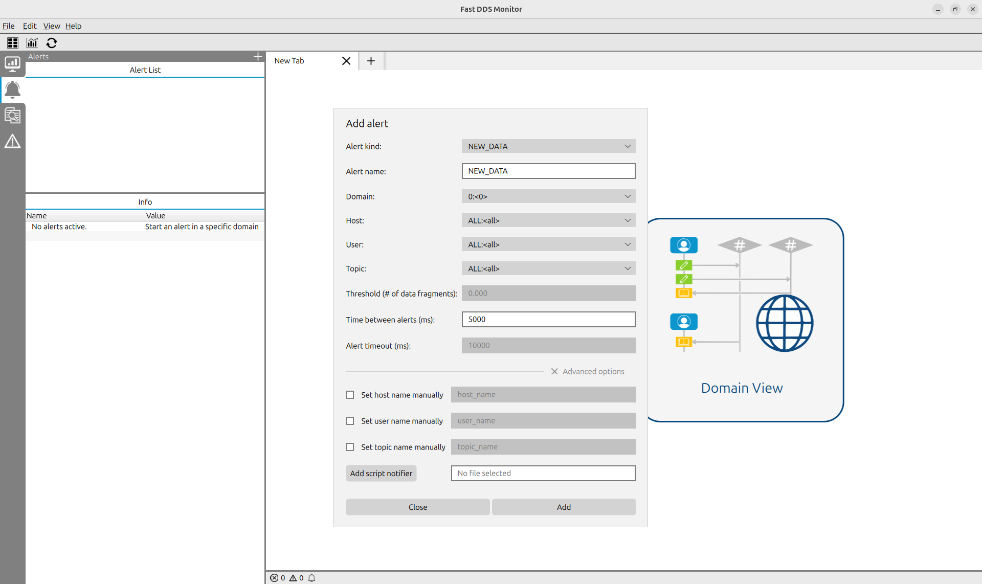
In this dialog, you can set the name of the alert, its type, the domain to monitor and the conditions for triggering the alert.

In general, all alerts filter the triggering entities using the fields host, user and topic. If any of these fields are left empty or the ALL option is selected, all entities will be compliant with that part of the filter. Note that the filter does not act like a regular expression, but like a simple equality check between strings. Note also that all 3 conditions must be met for an entity to be compliant with the alert filter.

If the alert type is NEW_DATA, the alert will be triggered when a positive DATA_COUNT is received from any entity that matches the fields host, user and topic.

If the alert type is NO_DATA, the alert will be triggered when a PUBLICATION_THROUGHPUT message is received from any entity that matches the fields host, user and topic and its value is lower than threshold.

If a timeout period is defined, the alert will trigger a timeout message with this periodicity. NEW_DATA alerts don’t support timeout due to their event-driven nature. However, the user can define a more relaxed polling time to collect timeout messages in the Edit->Alerts Configuration option from the upper menu.

Finally, if a script is provided, it will be executed every time the alert is triggered. Note that the script must have executable permissions in the host OS.

Once the alert is set up, it will appear in the list of alerts and its metadata will be shown below when clicked.

To remove an alert, just right-click on it and choose the Remove option.

3.3. DDS Monitor Pro

DDS Monitor Pro includes all the features of the open-source edition - everything demonstrated in the previous sections of this tutorial works in Pro exactly the same way. The sections below walk through the features that are exclusive to DDS Monitor Pro.

To showcase these capabilities a richer DDS network is needed than the minimal hello_world example. The main scenario in this tutorial uses the eProsima Shapes Demo, a graphical application that publishes and subscribes to colored geometric shapes on named DDS topics (Square, Circle, Triangle). Each shape sample carries four fields: color (a string), x, y, and shapesize (integers), which are ideal for live charts, spy views, and scatter plots. A separate scenario at the end of this section demonstrates the Image Pane .

3.3.1. Shapes Demo Scenario

eProsima Shapes Demo is available at https://github.com/eProsima/ShapesDemo. Follow the build and installation instructions in that repository before continuing. Once installed, two instances are needed to create the network used in this tutorial.

1. Open a terminal, source the eProsima Shapes Demo installation, and launch the first instance:

   source ~/shapes_demo_ws/install/setup.bash
   ShapesDemo
   

   In the Shapes Demo GUI, go to Options → Participant Configuration and make sure the Active statistics toggle is enabled (it is on by default) so the participant reports statistical data to the monitor. Then click Publish and create a Square publisher. Click Publish again and create a Circle publisher.

2. Open a second terminal and launch a second instance:

   source ~/shapes_demo_ws/install/setup.bash
   ShapesDemo
   

   In this second GUI, make sure Active statistics is enabled the same way under Options → Participant Configuration. Then click Subscribe and create a Square subscriber.

The DDS network now has three active endpoints on domain 0: a Square publisher and a Circle publisher in the first instance, and a Square subscriber in the second. Keep both Shapes Demo windows open throughout the tutorial.

3.3.2. DDS Monitor Pro Execution

Start DDS Monitor Pro. The start screen appears; press Start monitoring! to enter the main interface.

3.3.3. Initiate Monitoring

Once in the application, the initialization dialog asks you to select a monitoring mode. The Shapes Demo processes are running on domain 0. Select DDS Domain, enter 0, and click OK.

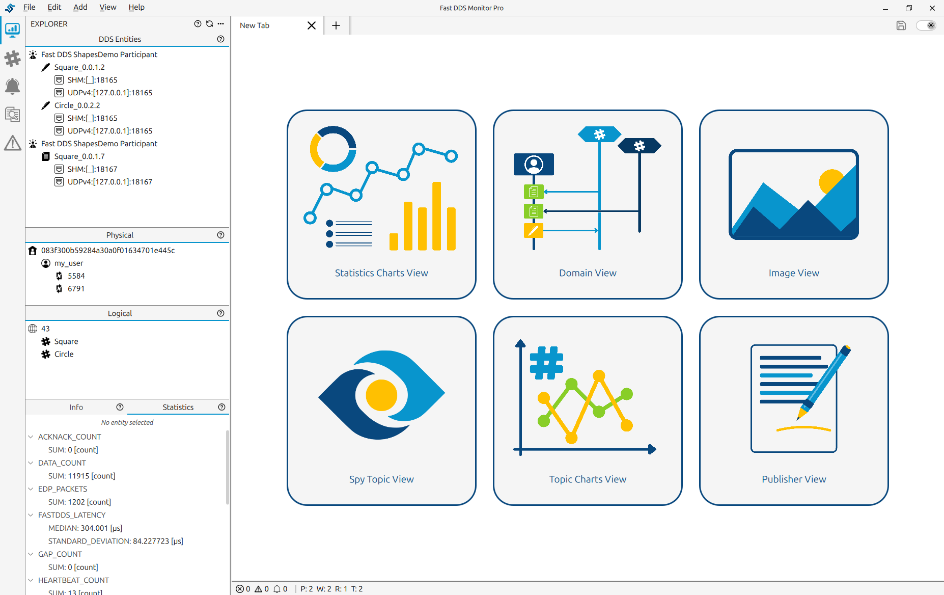
The monitor starts discovering entities. After a few seconds the Explorer Panel on the left shows the participants, writers, and reader created by the two Shapes Demo instances. Open all sub-panels by clicking the ··· button in the top-right corner of the Explorer Panel. The topics Square and Circle appear in the Logical panel under domain 0, and the host, users, and two processes appear in the Physical panel.

3.3.4. Explore the Domain View

Click Domain View in the main panel selector, or go to Add → Add Domain View, to see the DDS network as an interactive graph.

The graph shows both Shapes Demo processes as boxes inside the host. Each process contains its participant. The Square topic line runs vertically with a DataWriter arrow from the first process feeding into it and a DataReader arrow from the second process coming out - the full publish-subscribe connection is visible at a glance. The Circle topic line shows only a DataWriter arrow from the first process; it has no subscriber yet, so no reader arrow appears.

Right-click the Square topic line and choose Data type IDL view to open an IDL pane showing the ShapeType definition - the color, x, y, and shapesize fields are all visible. Close the IDL pane once you have inspected it.

Right-click the Square topic line and choose Filter topic graph to open a filtered view showing only the entities connected to that topic. A new tab opens with the Square publisher and subscriber - the Circle publisher is not shown since it is not related to the Square topic. Close the filtered tab and return to the full domain view.

Now let’s explore the visibility controls. Click the button in the Domain View pane header. The configuration panel opens on the right and shows DOMAIN GRAPH at the top. The panel lists all entities grouped into seven collapsible sections: TOPICS, HOSTS, USERS, PROCESSES, PARTICIPANTS, DATAWRITERS, and DATAREADERS. Each section header shows a visible/total count.

Hiding a process and its descendants

Expand the PROCESSES section. You will see the two Shapes Demo processes listed by their process ID or alias. Clear the checkbox next to one of them. That process disappears from the graph immediately - and so does everything it contained: its participant, the participant’s DataWriter or DataReader, and the locators associated with them. This is the container behavior: hiding a parent entity hides all its descendants automatically. Re-check the process to bring all its entities back at once.

Hiding and showing individual topics

Expand the TOPICS section. Both Square and Circle are listed. Clear the checkbox next to Circle. The Circle topic line vanishes from the graph along with its DataWriter arrow; the Square part of the graph is unaffected. Re-check Circle to restore it.

Use the Filter entities… search box at the top of the panel to find any entity by name quickly when the list is long.

Showing metatraffic

By default metatraffic is hidden. Go to View → Hide/Show Metatraffic to make it visible. A large number of new topic lines and endpoints appear in the graph - these are the internal statistics topics produced by the statistics module. Toggle the same menu item again to hide metatraffic and return to the clean graph.

To restore all manually hidden entities at once, use the ACTIONS button in the configuration panel and choose Show All Entities.

3.3.5. Topics Panel

Click the icon in the vertical icon bar on the far left of the window to open the Topics Panel. All discovered topics are listed here - Square and Circle are visible, together with the statistics metatraffic topics produced by the Fast DDS statistics module.

Click the small arrow next to Square to expand it. The fields of ShapeType are listed: color, x, y, and shapesize. The numeric fields x, y, and shapesize are interactive leaf nodes - they can be dragged onto an open chart to add a new series, or right-clicked to plot immediately.

3.3.6. Spy a Topic

Right-click Square in the Topics Panel and select Spy topic data. A Spy Topic View pane opens and immediately starts receiving live samples from the Square publisher.

Use the / button in the pane header to pause or resume the live feed without closing the pane. While paused, the last received sample stays visible for inspection.

3.3.7. Split Panes

DDS Monitor Pro can hold several views side by side within the same monitor tab. With the Spy pane already open, let’s split it to place a chart alongside it.

Click the … (three-dots) button in the Spy pane header and hover over Split right. A submenu appears listing all available pane types - select Topic Charts to open a Time Series Topic Chart to the right of the Spy pane.

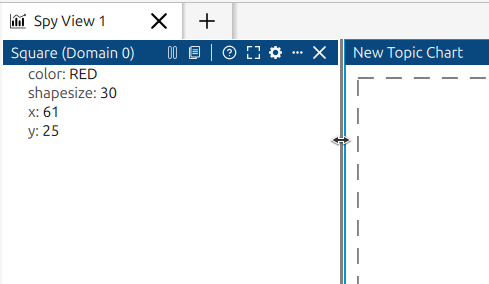
Drag the vertical divider between the panes to resize them as needed. The configuration panel opens automatically for the newly opened chart.

Up to six panes can be open in a single tab at the same time.

3.3.8. Plot a Topic Live Chart

With the Time Series Topic Chart pane open alongside the Spy pane, let’s configure it to track the Square’s position. The configuration panel already shows TIME SERIES CHART at the top.

Notice the PLOT MODE row: it has two buttons, Time Series and XY Chart, that switch this pane between the two chart types. Make sure Time Series is selected.

Under PANE SETTINGS:

• Domain – Domain 0.

• Time window – 60 seconds, so the last minute of data is visible.

• Max points – leave at 500.

• Click Apply & Reset Chart.

Under CHART NAME, type Square Position to label this chart.

Click Add Series in the SERIES section. The inline form expands: type Square in the Filter topics box. Select Square and wait a moment for the first sample to arrive - the field list populates with color, x, y, and shapesize. Click x and then click Add Series (or double-click x) to add it. Repeat and add y as a second series.

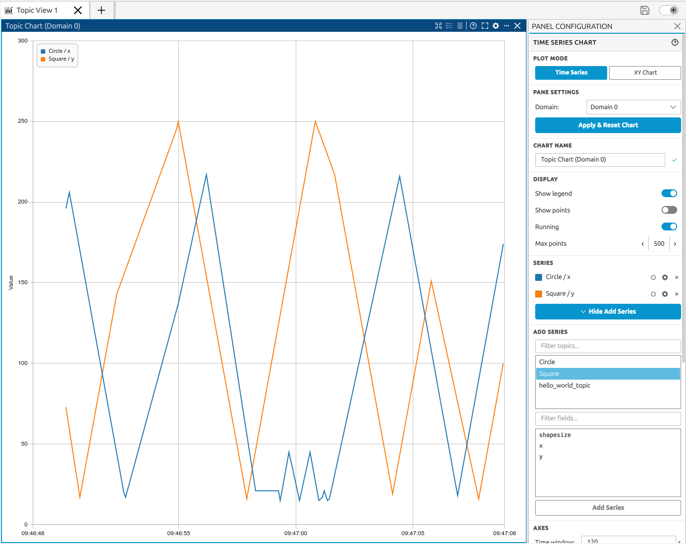
The chart now shows both the horizontal and vertical position of the square updating live as the shape bounces around the canvas. Under DISPLAY, enable Show legend to see the series names alongside their line colors.

You can also add series without using the configuration panel:

• From the Topics Panel - expand Square in the Topics Panel and drag the shapesize leaf directly onto the chart; a third series appears immediately.

• From the Spy pane - right-click the x field in the Spy pane and select Plot field to open a new chart for that field, or drag any numeric leaf from the sample tree onto an already-open chart to add it as a new series.

Click Reset View in the chart header at any time to return both axes to their default range after zooming or panning.

3.3.9. Plot an XY Chart

A Time Series chart shows each value changing over time. To see the shape’s trajectory - plotting x against y - switch to XY Chart mode.

Click in the Square Position chart header to open the configuration panel. Click the XY Chart button in the PLOT MODE row. The chart clears and the settings update for XY mode.

Under PANE SETTINGS:

• Domain – Domain 0.

• Max points – 150 to keep the scatter plot readable.

• Click Apply & Reset Chart.

Click Add XY Series in the SERIES section:

• X Axis Topic – select Square; X Field – select x.

• Y Axis Topic – select Square; Y Field – select y.

• Click Add XY Series.

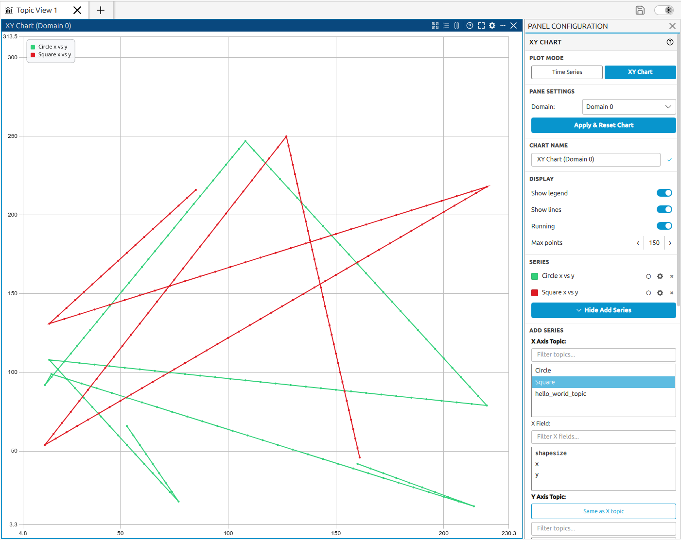
The scatter plot shows every position where the shape has been during the last 200 samples. As the Shapes Demo keeps running, new points appear and old ones drop off once the buffer is full. Because the shape bounces between the edges of the canvas, the point cloud outlines the boundaries of the Shapes Demo window as a rectangle.

When X and Y values come from different topics, each new X sample is paired with the most recent Y value, making it possible to plot correlations between any two numeric fields in the same domain.

3.3.10. Create a Custom Series

Beyond plotting topic fields directly, DDS Monitor Pro can plot a series computed from a JavaScript formula that combines one or more topic fields with your own constants. Let’s plot the Square’s distance from the origin, computed live from its x and y fields.

Open the Custom Series panel by clicking the icon in the vertical icon bar on the far left of the window, then click the button to create a new series. The formula editor opens in a central tab.

Fill in the editor as follows:

• Under SERIES NAME, type Square distance.

• Under DATA SOURCES, select Domain 0 and topic Square, pick the x field, type x in As var, and click Add Binding. Repeat for the y field with the variable name y.

• Under GLOBAL VARIABLES, add a variable named scale with the value 0.1.

• Under JAVASCRIPT FUNCTION BODY, write a formula that returns the scaled distance from the origin:

  return Math.sqrt(x * x + y * y) * scale;
  

Click Save & Exit. The new series appears in the Custom Series panel.

Open a Topic Chart (or reuse the Square Position chart) and drag the Square distance row from the Custom Series panel onto the chart, or right-click the row and choose Plot on chart. The computed series is plotted live alongside any other series, updating as new Square samples arrive.

Custom series definitions can be exported to a .json file with the button in the panel (or File → Export Custom Series…) and imported later with , independently of the workspace.

3.3.11. Statistics Charts

Beyond raw topic values, DDS Monitor Pro can also visualize pre-computed DDS statistics. Let’s add a live publication throughput chart for the Square publisher.

Click in the shortcuts toolbar, or go to Add → Add Statistics Chart. A new chart pane opens and the configuration panel shows STATISTICS CHART at the top.

Under PANE SETTINGS:

• Chart type – select Live (real-time).

• Data kind – choose PUBLICATION_THROUGHPUT.

• Time window – 120 seconds.

• Update period – 5 seconds.

• Click Apply & Restart.

Click Add Series in the SERIES section. The inline form expands with a Source entity selector. Choose the Square publisher participant as the source entity. Select MEAN for Statistics kind and click Add Series.

The series appears in the chart and updates every five seconds, showing the mean publication throughput of the Square publisher over time. Under CHART NAME, rename this chart to Throughput to make it easy to identify later.

Under AXES, enable Lock Y axis to keep the vertical scale stable. Under ACTIONS, click Export to CSV at any time to save the chart data to a file for offline analysis.

3.3.12. Enable and Disable Statistics

To save resources, DDS Monitor Pro only collects a statistic while something is using it. Creating the throughput chart in the previous section automatically enabled the PUBLICATION_THROUGHPUT reader behind the scenes. The Enable / Disable Statistics panel lets you see and control which statistics readers are active.

Click the icon in the vertical icon bar on the far left of the window to open the panel. Each statistic is listed with a toggle. The PUBLICATION_THROUGHPUT reader shows an information marker indicating it is active only because the throughput chart needs it - if you delete that chart, the reader is removed again automatically.

Alerts create statistics readers the same way. Let’s create one and watch its reader appear:

1. Click the icon in the shortcuts toolbar, or the + button in the Alerts Panel, to open the alert creation form.

2. Set an Alert kind of NEW_DATA (fires when a topic receives data), set the Topic filter to Square, and give the alert a name.

3. Click Create.

The NEW_DATA alert monitors the data count of the topic, so creating it automatically enables the DATA_COUNT reader. Return to the Enable / Disable Statistics panel and note that DATA_COUNT now appears active with an information marker, exactly like PUBLICATION_THROUGHPUT did for the chart - it stays only as long as the alert exists. See Alerts Panel for the full alert configuration reference.

Toggle a statistic on to keep its reader active permanently, even when no chart or alert uses it, so its data is always available. Toggle it off to stop collecting that statistic entirely. See Enable / Disable Statistics Panel for the full behavior, including which readers alerts create.

3.3.13. Publish Topic Data

The Publisher Pane lets you inject custom DDS samples directly from the monitor - without writing any code. Let’s publish a new Square shape and watch it appear in the Shapes Demo subscriber window.

Right-click Square in the Topics Panel and select Publish topic data. A Publisher Pane opens and the configuration panel shows PUBLISHER at the top.

The CURRENT TOPIC section shows the topic name (Square), the domain (Domain 0), the resolved type name (ShapeType), the publisher status, and a samples-sent counter.

Click Apply & Restart to attach the publisher to the Square topic. The pane body fills with an auto-generated form with one row per field in ShapeType. Click Randomize in the ACTIONS section of the configuration panel to fill all fields with random valid values automatically.

Click Publish once (the blue button at the bottom of the pane body, or Publish once in the ACTIONS section of the configuration panel) to send a single sample. The samples-sent counter in CURRENT TOPIC increments to 1. A shape with the randomized color, size, and position appears in the Shapes Demo instance that has the Square subscriber for the duration of one message lifetime.

To publish a continuous stream, enable Publish continuously in the CONTINUOUS section of the configuration panel and set Interval to 100 milliseconds. The shape stays refreshed at the same position for as long as continuous mode is active. Click the toggle again to stop publishing.

3.3.14. Register a Data Type

The Register Type View lets you supply a data type from its IDL so it can be used on topics whose type was never discovered on the network - for example, Safe DDS topics. Let’s use the ShapeType already on the network as a starting point to register a new type.

Open Add → Add Register Type View. A Register Type pane opens.

1. In the SELECT AN EXISTING TYPE OR START FROM SCRATCH dropdown, choose ShapeType. Its IDL loads into the editor.

2. In the REGISTER AS field, change the name to a new one, for example MyShapeType. Because this name is not a struct in the loaded IDL, the type is registered under it as an alias of ShapeType.

3. Click Save. The pane reports that the type was registered successfully.

The registered type is now available on every monitored domain and can be paired with any topic name. Although there is no topic using MyShapeType in this tutorial, you could now publish it on any topic from the Publisher Pane shown in the previous section - the publisher form would be built automatically from the registered type. See Register Type for the full workflow, including uploading IDL files with #include directives.

3.3.15. Add a Second Monitor

A notable feature of DDS Monitor Pro is the ability to run several independent monitors in the same window, each watching a different DDS environment. To showcase this, the next section displays a live image topic, so we run an image publisher on a separate domain (1) and add a second monitor tab for it.

Note

This tutorial does not ship an image publisher. Any DDS application that publishes an image-typed topic works - a ROS 2 node publishing sensor_msgs/msg/Image, or a Fast DDS application using the eProsima Fast DDS image types. A ready-to-use IDL for the latter is available in the monitor repository at resources/idl/FastDdsImage.idl; generate a type from it with Fast DDS Gen and publish frames on a topic in domain 1. See Image Pane for the full list of supported image schemas. The exact domain does not matter - any domain other than 0 keeps this scenario separate from the Shapes Demo network.

1. Start your image publisher on domain 1, publishing frames on an image topic.

2. In DDS Monitor Pro, open the File menu and select Initialize DDS Monitor. The initialization dialog appears. Enter 1, and click OK.

When you click the Domain View icon, there will appear a window allowing the user to choose a domain. Select domain 1. A second tab labeled with domain 1 appears in the main panel area alongside the first.

The Explorer Panel, entity lists, and the Topics Panel switch to show the entities from the second domain. The image topic appears in the Topics Panel and the image publisher’s participant is listed in the Explorer Panel. Click back to the domain 0 tab in the logical panel and everything returns to the Shapes Demo network instantly.

Each monitor operates entirely independently: entity discovery and data collection continue in the background regardless of which tab is currently visible.

3.3.16. View Live Image Data

The Image Pane renders live image frames from a DDS topic directly inside the monitor. The image publisher started in the previous section is already running on domain 1 and sending frames on the topic.

In the Topics Panel, right-click on the image topic and select Open image view. Alternatively, click the Image View button shown in the empty pane placeholder. A new Image Pane opens and the configuration panel shows IMAGE VIEW at the top.

Under CHANGE TOPIC, select Domain 1 and pick your image topic from the list (the list shows only the image topics). Click Apply & Reload.

The pane starts displaying frames as soon as the first one arrives. A metadata strip at the bottom of the pane shows the frame resolution, encoding, and a running total frame count.

Use the / button in the pane header to pause the stream. When paused, the last received frame stays visible so you can inspect it.

Under ACTIONS in the configuration panel, click Save Screenshot to save the current frame as a PNG file, or Copy Screenshot to copy it to the clipboard.

3.3.17. Map a Custom Image Topic

The Image Pane recognizes the standard ROS 2 and eProsima Fast DDS image types automatically. When a topic carries image data under a non-standard type - different field names, or a byte buffer with no width/height/encoding fields - you can still render it by mapping its fields manually.

Note

This step is optional and only applies when you have a topic whose type is not one of the recognized image schemas. To try it out, take the resources/idl/FastDdsImage.idl type from the previous section and rename its fields (for example width → cols, height → rows, encoding → color_format, step → line_size, data → pixels), then publish a topic with that modified type. The monitor will no longer auto-detect it as an image, which is exactly the case this mapping is for.

Open a new Image View (Add → Add Image View). In the NEW IMAGE VIEW form, if the image topic does not appear under IMAGE TOPIC, select it under CONFIGURE A CUSTOM TOPIC instead and click Configure as image topic. The CONFIGURE IMAGE TOPIC panel opens.

Choose the Visualization Mode (Raw image or Compressed image) and map each slot to a field of the topic type. For a raw image whose type names its fields cols, rows, color_format, line_size, and pixels instead of the standard names, map Width → cols, Height → rows, Encoding → color_format, Step / row stride → line_size, and Pixel data (bytes) → pixels. Each slot’s dropdown lists only fields of a compatible data type, and when the type has no suitable field you can enable Use a fixed value to supply a constant instead.

Click Save mapping. The topic becomes selectable under IMAGE TOPIC; select it and click Create Image View to render it just like a standard image topic. See Custom Image Topic for the full mapping reference.

3.3.18. Stop Monitoring a Domain

Now that we are done inspecting the image topic on domain 1, we no longer need that monitor. DDS Monitor Pro lets you stop monitoring a specific domain without closing its panes or affecting the other monitors.

Go to File → Stop Monitor and select domain 1 from the submenu. Monitoring of domain 1 stops: its entities are no longer tracked and its tab and panes remain open but become inactive, while the Shapes Demo monitor on domain 0 keeps running undisturbed. This is the reverse of Initialize DDS Monitor and is useful for freeing resources from a domain that is no longer of interest. See Stop Monitor for details.

3.3.19. Save and Restore a Workspace

After spending time setting up monitors, pane layouts, charts, and alert rules, it would be a waste to lose all that configuration when the application is closed. DDS Monitor Pro saves the complete session state to a workspace file and restores it exactly on the next launch.

Click the button in the toolbar at the top right of the window, or go to File → Save Workspace. A file dialog opens. Navigate to a suitable folder, type a name such as shapes_tutorial, and click Save. The file is written with the .fdmw extension.

To verify that the restore works, go to File → Load Workspace and select the shapes_tutorial.fdmw file. All monitor tabs, pane layouts, chart series, chart settings, alert rules, sidebar state, theme, and toolbar visibility are restored exactly as they were. Each monitor reopens in a waiting state and populates as the Shapes Demo processes are rediscovered.

Note

The statistics database is not stored in the workspace file. Entity discovery and data collection restart fresh on load; panes populate as DDS traffic is received after the workspace is applied.

3.3.20. Switch Theme

DDS Monitor Pro ships with Light and Dark themes. Every part of the interface (panels, charts, icons, dialogs, the title bar, and the menu bar) switches instantly when the theme is changed, with no restart required.

Go to View → Theme and select Dark, or use the / toggle in the shortcuts toolbar on the top right.

The entire application switches to the dark palette immediately. Charts use the same ten-color series palette in both themes so existing series remain easily distinguishable. Node and edge colors in the Domain View adapt automatically; entity status colors (green for alive, yellow for degraded, red for error) remain fixed so their meaning is always clear.

To revert, go to View → Theme and select Light.

The active theme is included in the workspace file and is restored the next time the shapes_tutorial.fdmw workspace is loaded.

3.3.21. Inspect a Recording (Offline Mode)

DDS Monitor Pro can open a previously captured DDS recording and inspect it with full playback control, instead of connecting to a live network. This is useful for analyzing an issue after it happened, or sharing a captured session with a colleague.

Note

This tutorial does not produce a recording. To obtain one, capture a DDS session with eProsima DDS Record & Replay, which saves DDS traffic to an .mcap database - for example, record the Shapes Demo network used earlier in this tutorial and then open the resulting file here. DDS Monitor Pro opens .mcap files and SQLite .db recordings.

Go to File → Open Recording… and select a recording file (an .mcap or SQLite .db file).

Note

Opening a recording never interrupts your live session. Because a monitor is already running in this window, the recording opens in a new, independent monitor application, leaving the live Shapes Demo monitor running untouched. You now have two separate monitor applications open at once, and closing one does not close the other.

A Select recording range dialog appears first; click Use full recording to load the whole capture, or pick a sub-range and click Apply range.

A playback bar appears at the bottom of the window with the recording name, the absolute start time and duration, a scrubbable timeline, play/pause, back/forward, a loop toggle, and a speed control. Drag the timeline (or left-drag directly on a chart plot) to move the playback cursor; the charts, spy, and image panes all update to show the data at that point. On a Topic Chart, each series’ value at the cursor is shown next to its entry in the legend, so the legend reads out the value of every series at the current playback point as you scrub.

See Offline Mode for the full list of playback controls and which panes are available while inspecting a recording.